Climate Modeling
The following four pages, on the Windows to the Universe web site, provide a basic overview of climate models. They are also written at a level that should be suitable for your students.
- Modeling the Future of Climate Change
- What Is a Climate Model?
- How Climate Models Work
- Accuracy and Uncertainty in Climate Models
|
Components of a Climate Model
Climate models include numerous elements of Earth's climate system, such as clouds, rainfall, sunlight, sea ice, oceans, evaporation, and so on. Click here to view an interactive diagram of the types of elements climate models contain; you can move your cursor over portions of the image to see descriptions of those elements. This diagram explicitly references NCAR's CCSM (Community Climate System Model), but the principles apply to other climate models.
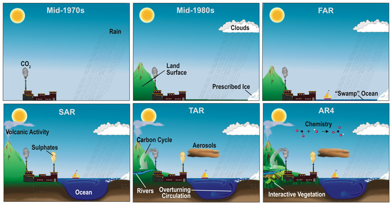
These diagrams depict the evolution of climate models, and the features included in them, over the years. Early models (in the 1970s) were relatively simple; they used just a few key features (incoming sunlight, rainfall, and CO2 concentration) to represent Earth's climate system. Models grew more sophisticated over time, incorporating clouds, land surface features, ice, and other elements into their calculations. Simple oceans were included in models beginning around the time of the IPCC's First Assessment Report (FAR) in the early 1990s; later models include more complex representations of oceans. Current climate models include clouds, a broader range of atmospheric constituents (sulphates, aerosols, etc.) and atmospheric chemistry, vegetation that exchanges gases with the atmosphere, and other features. The FAR, SAR, TAR, and AR4 labels on the diagrams indicate the models in use at the times of each of the four IPCC Assessment Reports. Credits: Images courtesy of the IPCC (AR4 WG 1 Chapter 1 page 99 Fig. 1.2). |
Resolution of Models
"Resolution" is an important concept in many types of modeling, including climate modeling. Spatial resolution specifies how large (in degrees of latitude and longitude or in km or miles) the grid cells in a model are. Temporal resolution refers to the size of the time steps used in models; how often (in simulated or "model time") calculations of the various properties being modeled are conducted (12-hour time steps are typical).
Models use grids of "cells" to establish the locations at which to perform calculations and thus make estimates of the traits (temperature, wind speed, etc.) that are of concern for that model. A typical climate model might have grid cells with a size of about 100 km (62 miles) on a side. Although we know that traits like temperature vary continuously across the face of the Earth, calculating such properties for the entire globe is beyond the reach of even the fastest supercomputers. Instead, the models typically use an algorithm that might be expressed as "calculate the temperature at a point, then move 100 km west and calculate temperature again; then move another 100 km west and repeat; once you've gone all the way around the globe, move 100 km north and repeat the process; and so on". In effect, the model places "virtual weather stations" at 100 km intervals and reports the calculated properties at each of the "weather stations". The "virtual weather stations" are located at the corners of the grid cells. So, for a model with 100 km resolution, we only know the predicted temperature (wind speed, etc.) at 100 km intervals. We can interpolate values in between "weather stations", but the reliability of such interpolations is limited.
Models can be generated with higher or lower resolutions. The grid cells could be reduced in size to 50 km, thus requiring more cells to cover Earth's surface and increasing resolution; or could be enlarged to 200 km, requiring fewer cells and decreasing resolution. More (and smaller) cells lead to increased computing time; there are simply more "virtual weather stations" at which atmospheric variables must be calculated. Higher resolution models provide much more detailed information, but at the cost of longer run times for the models on supercomputers.
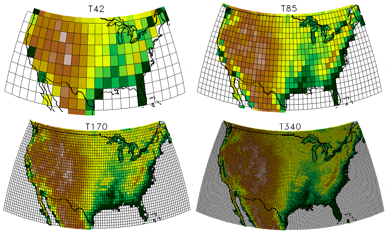
Climate models of the mid-1990s typically used grids similar to T42, which has grid cells of about 200 by 300 km (120 by 180 miles) at mid latitudes. The T85 resolution is typical for the models used in the IPCC's Fourth Assessment Report (AR4); its grid cells are about 100 by 150 km (60 by 90 miles) across at mid latitudes. The T170 and T340 grids represent future directions in modeling as new, more powerful supercomputers come online in the years ahead. Such models will be able to produce projections for regional climates that will be much finer than those we can currently generate. Remember, atmospheric models (including climate models) also have grid cells in the vertical direction, representing the variations that come with altitude in Earth's atmosphere. The images shown here just depict resolution in latitude and longitude directions. Credits: Images courtesy of Warren Washington, NCAR. |
Models grids for atmospheric (including climate) models are three dimensional; the grids must extend upward through our atmosphere. Early climate models typically had about 10 layers vertically; more recent ones often have about 30 layers. Because the atmosphere is so thin compared to the vast size of our planet, vertical layers are much closer together as compared to the horizontal dimensions of grid cells. Vertical layers might be spaced at 1 km intervals as compared to the 100 km intervals for horizontal spacing. However, the same principles regarding resolution apply; better resolution with smaller cells yields better results, but at the cost of increased computing time.
Climate modeling is a very computing-intensive field; climate modelers are always trying to get time on the newest, fastest supercomputers. As a general rule of thumb, increasing the resolution of a model by a factor of two means that about ten times as much computing power will be needed (or that the model will take ten times as long to run on the same computer). Most of this increase is simply a result of the larger number of "virtual weather stations" employed in the higher resolution model. For example, we might double the resolution of a model by decreasing grid cells from 100 x 100 km squares to 50 x 50 km squares and by increasing the number of vertical layers from 10 to 20. Each 3-D cell in the low resolution model would be replaced by eight cells in the higher resolution model (2 in latitude by 2 in longitude by 2 vertically = 8), so the higher resolution model might be expected to make about 8 times as many calculations.
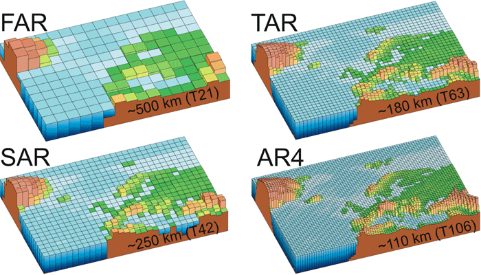
These images illustrate the typical spatial resolution used in state-of-the-art climate models around the times of each of the four IPCC Assessment Reports. Around the time of the First Assessment Report (FAR) in 1990, many climate models used a grid with cells of about 500 km (311 miles) on a side (upper left image). By the time of the the Second Assessment Report (SAR) in 1996, resolution had improved by a factor of two, producing grid cells 250 km (155 miles) on a side. Models references in the Third Assessment Report (TAR) in 2001 generally had reduced grid cells sizes to about 180 km (112 miles), while Fourth Assessment Report (AR4) models typically used a 110 km (68 mile) wide grid cell, further improving resolution. Vertical resolution is not depicted in these images, but has also improved over the years. Typical FAR models had a single-layer "slab ocean" and 10 atmospheric layers; AR4 models often include 30 layers in the oceans and another 30 in the atmosphere. Notice how elements of topography, such as the Alps Mountains, are shown in much greater detail in higher-resolution models. This allows such models to begin to make reasonable forecasts of regional climate in the future, a currently emerging capability. Credits: Image courtesy of the IPCC (AR4 WG 1 Chapter 1 page 113 Fig. 1.4). |
So far we've discussed spatial resolution; let's turn now to temporal resolution. Just as modelers must decide how close together in space to put the "virtual weather stations" at grid intersections, they must also decide how close together in time (that is, "virtual" or "model world" time) to make their calculations. As is the case with spatial resolution, there is a computing-time penalty to pay if the temporal resolution is too fine. If conditions in the model world are calculated too frequently, the model takes a very long time to run. If too much "model world" time passes between successive calculations, the model becomes inaccurate.
 Climate models are typically run with time steps of about 30 minutes; so, at this temporal resolution, the atmospheric properties in the modeled world are calculated each half hour. Climate models are often run out for a century into the future (sometimes for three or four centuries!). A typical climate model might, therefore, involve some 1,753,152 (the number of half-hours in a century) time steps. All model parameters (temperature, wind speed, humidity, etc.) would be calculated at each of the thousands to millions of grid points in the model at each of those time steps. That's a lot of calculating... sounds like a job for a supercomputer!
Climate modelers generally run a model for several "model years" before the time period they are interested in studying to get the model to stabilize at the initial equilibrium state. This "spin up" phase allows the modeled system to become stable before the modelers introduce conditions that alter the system, such as increased levels of carbon dioxide. It's a bit like running your car's engine for a while on a cold morning until the engine is warm and running smoothly. For example, a model might be run in "spin up" mode for 50 years with constant CO2 levels before beginning a simulation of the next 100 years with rising CO2 concentrations.


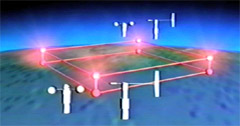
 This short segment (2 min. 14 sec.) of a video illustrates some of the basic elements of Global Climate Models (GCMs), including the construction of a grid upon which the model's calculations are based.


